Modelling animal home ranges

The goal of this project was to develop a mathematical model for animal behaviour that would result in realistic and stable home ranges. In this writeup I’ll explain my approach and the different models I tried.

The code for the project is in GitHub.

Approach

The home range of a herd of animals is simply the area where the animals regularly spend their time. Home ranges cover hunting grounds, nesting sites and breeding sites. This information is useful for researchers in understanding the group movement of animals.

My aim was to develop a model of individual animal movement that would result in a home range emerging.

A random walk model was used for its proven accuracy in simulating animal movement. The direction of the movement would be biased be the environment and presence of other animals.

Defining a Home Range

Before home range models can be evaluated, a definition for a home range is needed.

Data on real animals is typically collected in the form of distinct location coordinates at given times. The models developed for this project produce the same type of data: animal locations in time and space. In defining a home range the time data was discarded, leaving a set of coordinates.

Two main methods exist for relating this spatial data to a well-defined home range shape: minimum convex polygon fitting, and kernel density estimation.

Minimum Convex Polygon

The simplest method is to construct the smallest possible convex polygon (shown in black) around the locations visited by the animal (shown in blue):

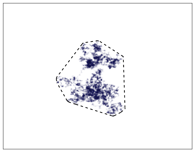
This is a well-defined method that doesn’t require subjectively choosing parameters. However, because the home range includes all locations, it tends to be larger than necessary. This effect is particularly noticeable if the animal ever wanders (perhaps before forming a stable home range):

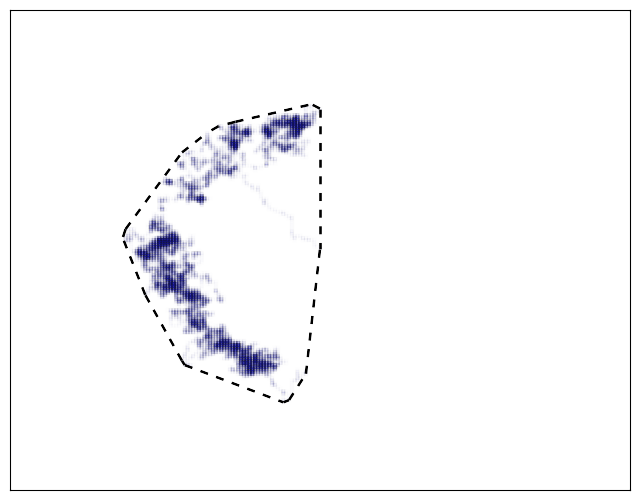
Wandering can be excluded by ignoring initial or uncommon points, but this introduces additional complexity and parameters, defeating the advantages of the method. Because this simulation project looks at animals converging to a stable home range, minimum convex polygon is not suitable as it cannot handle the initial travelling to a home range.

Kernel Density Estimation

It seems reasonable that an animal may occasionally move outside of its home range. If this is the case, a better approach to home range definition would be to consider where an animal spends most of its time, rather than all of it. Alternatively, this can be interpreted as how likely it is to find an animal at a given position.

This concept leads to a more robust method of defining home ranges: Kernel Density Estimation (KDE). Given a set of points, KDE produces a probability density function for the entire domain. Sampling the density function results in a set of points with similar distribution to those fed into the estimation.

Here’s what a KDE looks like on the same wandering walk that the convex hull failed to represent:

where darker red regions more likely to contain the animal, and therefore more likely to be in the home range. Choosing a threshold probability value gives a single line:

which appears to be a more accurate representation of a home range.

Random Walk Models

Each location in the grid can be assigned a quality q(x,y). This value represents the desirability of a certain position as perceived by the animal, and may incorporate factors such as food availability, predator territory, and climate. These qualities are combined into an environment matrix Q, with Qxy = q(x,y).

The environment quality is the only parameter for the walk, and it acts to bias the movement direction. At each timestep the animal moves to a neighbouring grid cell with a probability proportional to the neighbouring cells’ respective quality.

So now the model of animal movement becomes a method for defining the quality of the environment.

Environment Quality

2D environments were created by taking random noise:

and applying Gaussian blur:

to make the variation more realistic. In this example, dark areas have high quality and attract the animals - which might represent an area with plentiful food or good shelter. Animals are unlikely to move towards the lighter white areas, which might represent a predator’s territory or dangerous terrain.

Let’s release a herd of 10 animals into the centre one of these environments and see what happens:

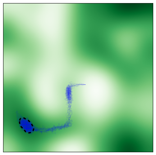
They travel together to a local maximum, with their travel history shown again in blue. The model is a form of gradient descent, where the environment is the objective function and the random walk adds stochasticity to the optimisation.

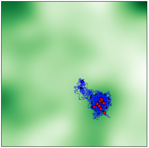
However, this nice convergence is not always seen. Multiple animal convergence depends on the steepness, size, and uniqueness of the local maximum. Here’s different random environment, with the final positions of the animals shown in red:

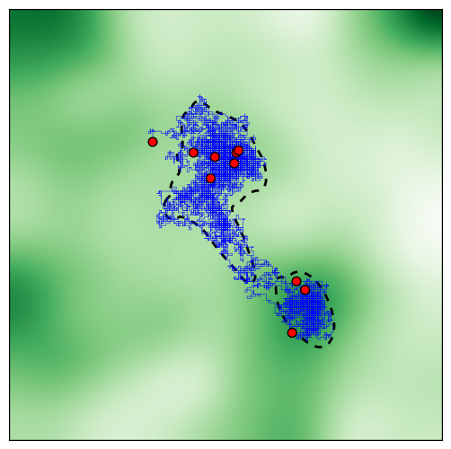
Because of the two local maxima found on either side of the starting point, the herd splits and animals end up in different areas with a fractured home range. This seems like an unlikely result; it’s difficult to imagine a small group of tightly packed herding animals splitting in opposite directions.

It seems that simply heading towards desirable areas isn’t enough for home ranges to emerge.

Olfactory Model

Some form of animal interaction is needed, which is often realised in nature by leaving some sort of scent. This scent diffuses and decays over time, which can be considered as a dynamic environment quality that changes each iteration.

I assumed the animals produced scent at their current position at a constant rate. The scent was then spread according to the 2D diffusion equation

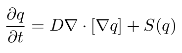
which is total overkill for this project, but I wanted to get some use out of my fluid dynamics course.

The resulting model causes the animals to remain close to each other because they are attracted to the scent of the other animals. They tend to follow each other because of the scent of their tracks. And because the scent is slowly diffusing they remain largely in the same place.

Here’s how the scent attraction quality looks like at a particular point in time:

Combined model

The next logical step is to combine the environment quality model with scent attraction. This is done by combining the two qualities:

with a weighting m for each one. The result looks good:

This is the same environment that the animals failed on with the basic environment model. And now they remain together in a stable home range. Success!

Stray Observations:

• This is essentially a 2D optimisation problem, which pops up a lot in mathematics. It’s cool to see that animals have to deal with this stuff too.